Community Diversity (skbio.diversity)#
This module provides functionality for analyzing biodiversity of communities – groups of organisms living in the same area. It implements various metrics of alpha (within-community) and beta (between-community) diversity, and provides “driver functions” for computing alpha and beta diversity for an entire data table. Additional utilities are provided to support discovery of available diversity metrics. While diversity metrics were originally designed to study biological communities, they can be generalized to the analysis of various biological data types.
See an Introduction to community data and diversity metrics and a Tutorial for performing community diversity analyses using scikit-bio.
Alpha diversity#
Alpha diversity metrics
Alpha diversity measures (skbio.diversity.alpha) |
|
List scikit-bio's alpha diversity metrics. |
Driver function
Compute alpha diversity for one or more samples. |
Beta diversity#
Beta diversity metrics
Beta diversity measures (skbio.diversity.beta) |
|
List scikit-bio's beta diversity metrics. |
Driver functions
Compute distances between all pairs of samples. |
|
Compute distances only between specified ID pairs. |
|
Perform a block-decomposition beta diversity calculation. |
Utility functions#
Index tree and convert counts to np.array in corresponding order. |
Introduction#
A community (i.e., sample) is represented by a vector of frequencies of taxa within the sample. The term “taxon” (plural: “taxa”) describes a group of biologically related organisms that constitute a unit in the community. Taxa are usually defined at a uniform taxonomic rank, such as species, genus or family. In community ecology, taxon is usually referred to as “species” (singular = plural), but its definition is not limited to species as a taxonomic rank. The term “taxonomic group” is a synonym of taxon in many situations.
In scikit-bio, the term “taxon/taxa” is used very loosely, as these can in practice represent diverse feature types including organisms, genes, and metabolites. The term “sample” is also loosely defined for these purposes. These are intended to represent a single unit of sampling, and as such what a single sample represents can vary widely. For example, in a microbiome survey, these could represent all 16S rRNA gene sequences from a single oral swab. In a comparative genomics study on the other hand, a sample could represent an individual organism’s genome.
Note
Previous versions of scikit-bio referred to taxon as operational taxonomic unit (OTU), a historically important term in microbiome research. However, as the field advances and the research targets diverge (e.g., amplicon sequence variant, or ASV), a more generic term such as “taxon” becomes more appropriate. Therefore, the term OTU was replaced by taxon in scikit-bio 0.6.0.
Each frequency in a given vector represents the number of individuals observed
for a particular taxon. We will refer to the frequencies associated with a
single sample as a counts vector or counts throughout the documentation.
Counts vectors are array_like: anything that can be converted into a 1-D
array is acceptable input. For example, you can provide a NumPy array or a
native Python list and the results will be identical.
The driver functions alpha_diversity and beta_diversity are
designed to compute alpha diversity for one or more samples, or beta diversity
for one or more pairs of samples. The driver functions accept a matrix
containing vectors of frequencies of taxa within each sample. Each row in the
matrix represents a single sample’s count vector, so that rows represent
samples and columns represent taxa.
Some diversity metrics incorporate relationships between the taxa in their
computation through reference to a phylogenetic tree. These metrics
additionally take a TreeNode object and a list of taxa mapping
the values in the counts vector to tips in the tree.
The driver functions are optimized so that computing a diversity metric more
than one time (i.e., for more than one sample for alpha diversity metrics, or
more than one pair of samples for beta diversity metrics) is often much faster
than repeated calls to the metric. For this reason, the driver functions take
matrices of counts vectors rather than a single counts vector for alpha
diversity metrics or two counts vectors for beta diversity metrics. The
alpha_diversity driver function will thus compute alpha diversity for all
counts vectors in the matrix, and the beta_diversity driver function will
compute beta diversity for all pairs of counts vectors in the matrix.
Input validation#
The driver functions perform validation of input by default. Validation can be
slow so it is possible to disable this step by passing validate=False. This
can be dangerous however. If invalid input is encountered when validation is
disabled it can result in difficult-to-interpret error messages or incorrect
results. We therefore recommend that users are careful to ensure that their
input data is valid before disabling validation.
The conditions that the driver functions validate follow. If disabling validation, users should be confident that these conditions are met.
the data in the counts vectors can be safely cast to integers
there are no negative values in the counts vectors
each counts vector is one dimensional
the counts matrix is two dimensional
all counts vectors are of equal length
Additionally, if a phylogenetic diversity metric is being computed, the following conditions are also confirmed:
the provided taxa are all unique
the length of each counts vector is equal to the number of taxa
the provided tree is rooted
the tree has more than one node
all nodes in the provided tree except for the root node have branch lengths
all tip names in the provided tree are unique
all provided taxa correspond to tip names in the provided tree
Count vectors#
There are different ways that count vectors are represented in the ecological literature and in related software. The diversity measures provided here always assume that the input contains abundance data: each count represents the number of individuals observed for a particular taxon in the sample. For example, if you have two taxa, where three individuals were observed from the first taxon and only a single individual was observed from the second taxon, you could represent this data in the following forms (among others).
As a vector of counts. This is the expected type of input for the diversity measures in this module. There are 3 individuals from the taxon at index 0, and 1 individual from the taxon at index 1:
>>> counts = [3, 1]
As a vector of indices. The taxon at index 0 is observed 3 times, while the taxon at index 1 is observed 1 time:
>>> indices = [0, 0, 0, 1]
As a vector of frequencies. We have 1 taxon that is a singleton and 1 taxon that is a tripleton. We do not have any 0-tons or doubletons:
>>> frequencies = [0, 1, 0, 1]
Always use the first representation (a counts vector) with this module.
Specifying a diversity metric#
The driver functions take a parameter, metric, that specifies which
diversity metric should be applied. The value that you provide for metric
can be either a string (e.g., "faith_pd") or a function (e.g.,
faith_pd). The metric should generally be passed as a string,
as this often uses an optimized version of the metric. For example, passing
metric="faith_pd" (a string) to alpha_diversity will be tens of times
faster than passing metric=faith_pd (a function) when computing Faith’s PD
on about 100 samples. Similarly, passing metric="unweighted_unifrac" (a
string) will be hundreds of times faster than passing
metric=unweighted_unifrac (a function) when computing unweighted UniFrac
on about 100 samples. The latter may be faster if computing only one alpha or
beta diversity value, but in these cases the run times will likely be so small
that the difference will be negligible. We therefore recommend that you
always pass the metric as a string when possible.
Passing a metric as a string will not be possible if the metric you’d like to
run is not one that scikit-bio knows about. This might be the case, for
example, if you’re applying a custom metric that you’ve developed. To discover
the metric names that scikit-bio knows about as strings that can be passed as
metric to alpha_diversity or beta_diversity, you can call
get_alpha_diversity_metrics or get_beta_diversity_metrics,
respectively. These functions return lists of alpha and beta diversity metrics
that are implemented in scikit-bio. There may be additional metrics that can be
passed as strings which won’t be listed here, such as those implemented in
SciPy’s pdist.
Tutorial#
Create a matrix containing 6 samples (rows) and 7 taxa (columns):
>>> data = [[23, 64, 14, 0, 0, 3, 1],
...         [0, 3, 35, 42, 0, 12, 1],
...         [0, 5, 5, 0, 40, 40, 0],
...         [44, 35, 9, 0, 1, 0, 0],
...         [0, 2, 8, 0, 35, 45, 1],
...         [0, 0, 25, 35, 0, 19, 0]]
>>> ids = list('ABCDEF')
First, we’ll compute \(S_{obs}\), an alpha diversity metric, for each
sample using the alpha_diversity driver function:
>>> from skbio.diversity import alpha_diversity
>>> adiv_sobs = alpha_diversity('sobs', data, ids)
>>> adiv_sobs
A    5
B    5
C    4
D    4
E    5
F    3
dtype: ...
Next we’ll compute Faith’s PD on the same samples. Since this is a phylogenetic diversity metric, we’ll first create a tree and an ordered list of taxa.
>>> from skbio import TreeNode
>>> from io import StringIO
>>> tree = TreeNode.read(StringIO(
...                      '(((((U1:0.5,U2:0.5):0.5,U3:1.0):1.0):0.0,'
...                      '(U4:0.75,(U5:0.5,(U6:0.5,U7:0.5):0.5):'
...                      '0.5):1.25):0.0)root;'))
>>> taxa = ['U1', 'U2', 'U3', 'U4', 'U5', 'U6', 'U7']
>>> adiv_faith_pd = alpha_diversity('faith_pd', data, ids=ids,
...                                 taxa=taxa, tree=tree)
>>> adiv_faith_pd
A    6.75
B    7.00
C    6.25
D    5.75
E    6.75
F    5.50
dtype: float64
Now we’ll compute Bray-Curtis distances, a beta diversity metric, between
all pairs of samples. Notice that the data and ids parameters
provided to beta_diversity are the same as those provided to
alpha_diversity.
>>> from skbio.diversity import beta_diversity
>>> bc_dm = beta_diversity("braycurtis", data, ids)
>>> print(bc_dm)
6x6 distance matrix
IDs:
'A', 'B', 'C', 'D', 'E', 'F'
Data:
[[ 0.          0.78787879  0.86666667  0.30927835  0.85714286  0.81521739]
 [ 0.78787879  0.          0.78142077  0.86813187  0.75        0.1627907 ]
 [ 0.86666667  0.78142077  0.          0.87709497  0.09392265  0.71597633]
 [ 0.30927835  0.86813187  0.87709497  0.          0.87777778  0.89285714]
 [ 0.85714286  0.75        0.09392265  0.87777778  0.          0.68235294]
 [ 0.81521739  0.1627907   0.71597633  0.89285714  0.68235294  0.        ]]
Next, we’ll compute weighted UniFrac distances between all pairs of samples.
Because weighted UniFrac is a phylogenetic beta diversity metric, we’ll need
to pass the skbio.TreeNode and list of taxa that we created above.
Again, these are the same values that were provided to alpha_diversity.
>>> wu_dm = beta_diversity("weighted_unifrac", data, ids, tree=tree,
...                        taxa=taxa)
>>> print(wu_dm)
6x6 distance matrix
IDs:
'A', 'B', 'C', 'D', 'E', 'F'
Data:
[[ 0.          2.77549923  3.82857143  0.42512039  3.8547619   3.10937312]
 [ 2.77549923  0.          2.26433692  2.98435423  2.24270353  0.46774194]
 [ 3.82857143  2.26433692  0.          3.95224719  0.16025641  1.86111111]
 [ 0.42512039  2.98435423  3.95224719  0.          3.98796148  3.30870431]
 [ 3.8547619   2.24270353  0.16025641  3.98796148  0.          1.82967033]
 [ 3.10937312  0.46774194  1.86111111  3.30870431  1.82967033  0.        ]]
Next we’ll do some work with these beta diversity distance matrices. First, we’ll determine if the UniFrac and Bray-Curtis distance matrices are significantly correlated by computing the Mantel correlation between them. Then we’ll determine if the p-value is significant based on an alpha of 0.05.
>>> from skbio.stats.distance import mantel
>>> r, p_value, n = mantel(wu_dm, bc_dm)
>>> print(r)
0.922404392093
>>> alpha = 0.05
>>> print(p_value < alpha)
True
Next, we’ll perform principal coordinates analysis (PCoA) on our weighted UniFrac distance matrix.
>>> from skbio.stats.ordination import pcoa
>>> wu_pc = pcoa(wu_dm)
PCoA plots are only really interesting in the context of sample metadata, so let’s define some before we visualize these results.
>>> import pandas as pd
>>> sample_md = pd.DataFrame([
...    ['gut', 's1'],
...    ['skin', 's1'],
...    ['tongue', 's1'],
...    ['gut', 's2'],
...    ['tongue', 's2'],
...    ['skin', 's2']],
...    index=['A', 'B', 'C', 'D', 'E', 'F'],
...    columns=['body_site', 'subject'])
>>> sample_md
  body_site subject
A       gut      s1
B      skin      s1
C    tongue      s1
D       gut      s2
E    tongue      s2
F      skin      s2
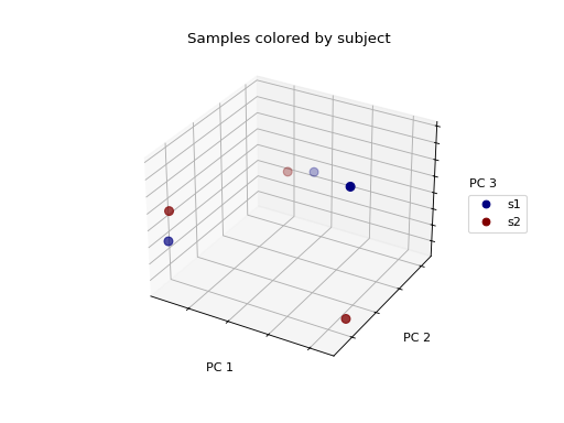
Now let’s plot our PCoA results, coloring each sample by the subject it was taken from:
>>> fig = wu_pc.plot(
...     sample_md, 'subject',
...     axis_labels=('PC 1', 'PC 2', 'PC 3'),
...     title='Samples colored by subject',
...     cmap='jet', s=50
... )

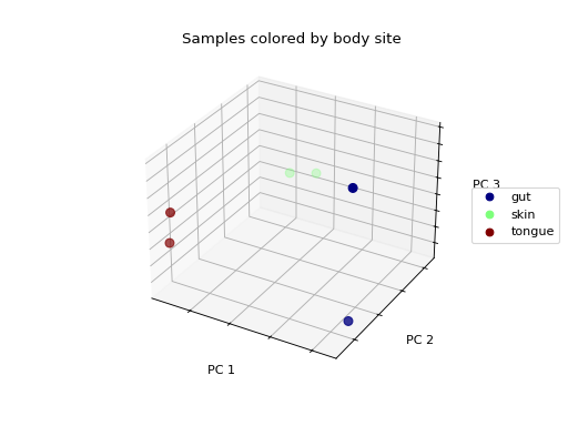
We don’t see any clustering/grouping of samples. If we were to instead color the samples by the body site they were taken from, we see that the samples from the same body site (those that are colored the same) appear to be closer to one another in the 3-D space then they are to samples from other body sites.
>>> fig = wu_pc.plot(
...     sample_md, 'body_site',
...     axis_labels=('PC 1', 'PC 2', 'PC 3'),
...     title='Samples colored by body site',
...     cmap='jet', s=50
... )

Ordination techniques, such as PCoA, are useful for exploratory analysis. The next step is to quantify the strength of the grouping/clustering that we see in ordination plots. There are many statistical methods available to accomplish this; many operate on distance matrices. Let’s use ANOSIM to quantify the strength of the clustering we see in the ordination plots above, using our weighted UniFrac distance matrix and sample metadata.
First test the grouping of samples by subject:
>>> from skbio.stats.distance import anosim
>>> results = anosim(wu_dm, sample_md, column='subject', permutations=999)
>>> results['test statistic']
-0.33333333333333331
>>> results['p-value'] < 0.1
False
The negative value of ANOSIM’s R statistic indicates anti-clustering and the p-value is insignificant at an alpha of 0.1.
Now let’s test the grouping of samples by body site:
>>> results = anosim(wu_dm, sample_md, column='body_site', permutations=999)
>>> results['test statistic']
1.0
>>> results['p-value'] < 0.1
True
The R statistic indicates strong separation of samples based on body site. The p-value is significant at an alpha of 0.1.
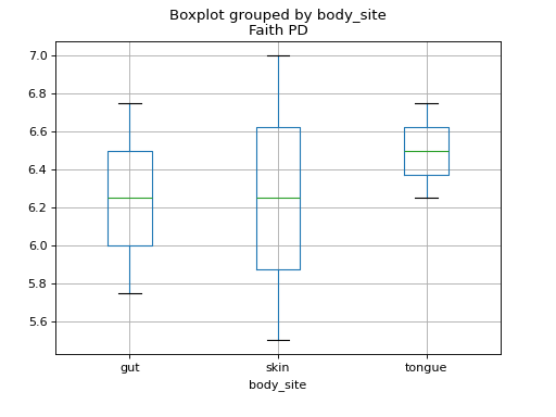
We can also explore the alpha diversity in the context of sample metadata.
To do this, let’s add the observed richness and Faith’s PD metrics to our
sample metadata. This is straight-forward because alpha_diversity
returns a Pandas Series object, and we’re representing our sample
metadata in a Pandas DataFrame object.
>>> sample_md['Obs. richness'] = adiv_sobs
>>> sample_md['Faith PD'] = adiv_faith_pd
>>> sample_md
  body_site subject  Obs. richness  Faith PD
A       gut      s1              5      6.75
B      skin      s1              5      7.00
C    tongue      s1              4      6.25
D       gut      s2              4      5.75
E    tongue      s2              5      6.75
F      skin      s2              3      5.50
We can investigate these alpha diversity data in the context of our metadata categories. For example, we can generate boxplots showing Faith PD by body site.
>>> fig = sample_md.boxplot(column='Faith PD', by='body_site')

We can also compute Spearman correlations between all pairs of columns in
this DataFrame. Since our alpha diversity metrics are the only two
numeric columns (and thus the only columns for which Spearman correlation
is relevant), this will give us a symmetric 2x2 correlation matrix.
>>> sample_md.corr(method="spearman", numeric_only=True)
               Obs. richness  Faith PD
Obs. richness       1.000000  0.939336
Faith PD            0.939336  1.000000